CPC Afterburn: Active Inference and the Bayesian Brain

Hey everyone, and welcome back to the CPC Afterburn series! In our last post, we explored the fascinating world of Predictive Coding. Today, we’re going to level up and dive into some of the core principles that form the foundation of computational psychiatry and modern AI: Bayesian Inference, the Markov Decision Process (MDP), the Free-Energy Principle, and Active Inference.
As software engineers, we’re used to building systems that follow explicit instructions. But what if we could build systems that learn and act more like the human brain? These concepts provide a powerful framework for thinking about how the brain—and intelligent agents in general—might handle uncertainty, make decisions, and navigate the world.
Bayesian Inference: The Brain’s Belief-Updating Algorithm
At its core, the brain is a belief-updating machine. It starts with a prior assumption, gathers evidence through the senses, and then updates its beliefs. This is the essence of Bayesian Inference.
For a software engineer, this is directly analogous to building a system that learns from user data. Imagine you’re running an A/B test for three different versions of a “Buy” button on your website. You don’t know which is best, so you start with the assumption that they are all equally effective. As users click (or don’t click), you gather data and continuously update your belief about the true click-through rate of each button.
This leads to the classic “explore-exploit” dilemma: should you keep exploring all options to get more data, or exploit the one that currently seems the best?
A beautiful Bayesian solution to this is Thompson Sampling. Each button’s “true” click-through rate is modeled as a probability distribution (our belief). To make a decision, we simply take one random sample from each distribution and choose the button with the highest sample. The result of that choice is then used to update the distribution. This naturally balances exploration and exploitation.
Let’s model this with a “Multi-Armed Bandit” problem, where each button is a slot machine with a different, unknown win rate.
import numpy as np
import matplotlib.pyplot as plt
from scipy.stats import beta

# --- The Multi-Armed Bandit Simulation ---

# Define the true, unknown click-through rates for 3 buttons
true_probabilities = [0.25, 0.55, 0.60]
# We'll use the Beta distribution to model our belief about each button's rate.
# We start with a "uniform prior" (alpha=1, beta=1), meaning any rate is equally likely.
# alpha = successes + 1, beta = failures + 1
button_beliefs = np.ones((len(true_probabilities), 2)) # [[1,1], [1,1], [1,1]]

num_trials = 1000
total_rewards = 0
chosen_buttons = []

for i in range(num_trials):
    # 1. Thompson Sampling: Sample from the posterior of each button's belief
    sampled_beliefs = [np.random.beta(a, b) for a, b in button_beliefs]

    # 2. Exploit: Choose the button with the highest sampled belief
    chosen_button = np.argmax(sampled_beliefs)
    chosen_buttons.append(chosen_button)

    # 3. Explore: "Pull the arm" of the chosen button and get a result
    # We simulate a click based on the true probability
    reward = 1 if np.random.random() < true_probabilities[chosen_button] else 0
    total_rewards += reward

    # 4. Bayesian Update: Update our belief for the button we chose
    if reward == 1:
        button_beliefs[chosen_button][0] += 1 # Increment alpha (successes)
    else:
        button_beliefs[chosen_button][1] += 1 # Increment beta (failures)

# --- Analysis and Visualization ---
estimated_rates = [a / (a + b) for a, b in button_beliefs]

print(f"Simulation complete after {num_trials} trials.")
print(f"Total rewards: {total_rewards}\n")
for i in range(len(true_probabilities)):
    print(f"Button {i+1}: True Rate={true_probabilities[i]:.2f}, "
          f"Estimated Rate={estimated_rates[i]:.2f}, "
          f"Chosen {chosen_buttons.count(i)} times.")

# Plot the posterior distributions
x = np.linspace(0, 1, 200)
plt.figure(figsize=(10, 5))
for i, (a, b) in enumerate(button_beliefs):
    plt.plot(x, beta.pdf(x, a, b), label=f'Button {i+1} Belief (True Rate: {true_probabilities[i]})')
plt.title("Posterior Beliefs about Button Click-Through Rates")
plt.xlabel("Click-Through Rate")
plt.ylabel("Density")
plt.legend()
plt.show()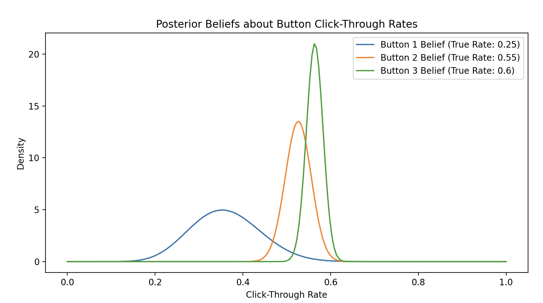
When you run this, you’ll see the agent quickly learns to favor the best button (Button 3), but still occasionally tries the others. The final plot shows the agent’s updated beliefs: sharp, confident peaks centered around the true win rates. This is a system that actively minimizes its own uncertainty to maximize rewards—a core idea we’ll see again.
Markov Decision Process (MDP): A Framework for Decision-Making
If Bayesian Inference is about updating beliefs, the Markov Decision Process (MDP) is a powerful framework for using those beliefs to plan a sequence of actions. It’s the cornerstone of reinforcement learning.
As a software engineer, think of an MDP as the formal specification for any goal-oriented agent, whether it’s a Roomba cleaning a floor, a character navigating a game level, or a system managing cloud resources. It consists of:
- States (S): The different situations the agent can be in (e.g., grid coordinates).
- Actions (A): What the agent can do in each state (e.g., move ‘Up’, ‘Down’).
- Transition Model P(s’ | s, a): The rules of the world. “If you’re in state
sand take actiona, what’s the probability of ending up in states'?” - Reward Function R(s): The goal. What’s the reward for entering state
s?
The agent’s goal is to find a policy ()—a mapping from states to actions—that maximizes its cumulative future reward.
Instead of just defining an MDP, let’s solve one. We’ll create a simple grid world and use Value Iteration, a classic algorithm that finds the optimal policy. It works by calculating the “value” of being in each state, which is the total reward an agent can expect to get if it starts there and acts optimally.
import numpy as np

# --- MDP Definition: A 3x4 Grid World ---
# 'S' = Start, 'G' = Goal (reward), 'X' = Obstacle (penalty)
# [[' ', ' ', ' ', 'G'],
#  [' ', 'X', ' ', ' '],
#  ['S', ' ', ' ', ' ']]
grid_shape = (3, 4)
goal_state, obstacle_state, start_state = (0, 3), (1, 1), (2, 0)
states = [(r, c) for r in range(grid_shape[0]) for c in range(grid_shape[1])]
actions = ['U', 'D', 'L', 'R']
gamma = 0.9 # Discount factor for future rewards

# --- Reward and Transition Logic ---
def get_reward(state):
    if state == goal_state: return 10
    if state == obstacle_state: return -10
    return -0.1 # Small cost for each step to encourage efficiency

def transition(state, action):
    if state in [goal_state, obstacle_state]: return state
    row, column = state
    if action == 'U': row = max(0, row - 1)
    if action == 'D': row = min(grid_shape[0] - 1, row + 1)
    if action == 'L': column = max(0, column - 1)
    if action == 'R': column = min(grid_shape[1] - 1, column + 1)
    # The agent cannot move into the obstacle from an adjacent square
    return state if (r, c) == obstacle_state else (r, c)

# --- Value Iteration Algorithm ---
def value_iteration():
    V = {s: 0 for s in states} # Initialize value of all states to 0
    while True:
        delta = 0
        for s in states:
            if s in [goal_state, obstacle_state]: continue
            old_v = V[s]
            # Bellman Equation: V(s) = max_a Σ [ R(s') + γ * V(s') ]
            action_values = []
            for a in actions:
                next_s = transition(s, a)
                action_values.append(get_reward(next_s) + gamma * V[next_s])
            V[s] = max(action_values)
            delta = max(delta, abs(old_v - V[s]))
        if delta < 1e-5: # Convergence check
            break
    return V

# --- Derive the Optimal Policy from the Value Function ---
def get_policy(V):
    policy = {s: '' for s in states}
    for s in states:
        if s in [goal_state, obstacle_state]: continue
        action_values = {}
        for a in actions:
            next_s = transition(s, a)
            action_values[a] = get_reward(next_s) + gamma * V[next_s]
        policy[s] = max(action_values, key=action_values.get)
    return policy

# --- Run and Display ---
value_function = value_iteration()
optimal_policy = get_policy(value_function)

print("Optimal Policy (Agent's 'Plan'):")
policy_grid = np.full(grid_shape, ' ', dtype=str)
for state, action in optimal_policy.items():
    if state == goal_state: policy_grid[state] = 'G'
    elif state == obstacle_state: policy_grid[state] = 'X'
    else: policy_grid[state] = {'U':'↑', 'D':'↓', 'L':'←', 'R':'→'}.get(action, ' ')

print(policy_grid)
Output:
Optimal Policy (Agent's 'Plan'):
[['→' '→' '→' 'G']
 ['↑' 'X' '↑' '↑']
 ['↑' '→' '↑' '↑']]
The output of this code is a complete plan. It doesn’t just define the world; it solves it, showing the best action to take from any square on the grid to reach the goal most efficiently. This is far more powerful—it’s a generative model of behavior. The agent now has a set of predictions about what to do to reach a desired state, which is a perfect segue into our next topics.
The Free-Energy Principle: The Brain’s Grand Unifying Theory?
Now, let’s get a bit more abstract. The Free-Energy Principle is a theory from Karl Friston that proposes a single, underlying principle for all self-organizing systems, including the brain. It states that these systems must minimize a quantity called “variational free energy.”
In simple terms, free energy is a measure of surprise or prediction error. A brain that is good at minimizing free energy is good at predicting its sensory inputs. Think of it like a highly optimized compression algorithm. A good compression algorithm is one that has a good model of the data, and therefore is not “surprised” by it.
For a software engineer, this is like minimizing the loss function of a machine learning model. The goal is to adjust the model’s parameters (its internal beliefs) to minimize the difference between the model’s predictions and the actual data.
Active Inference: Perception and Action as Two Sides of the Same Coin
So, how does the brain minimize free energy? Through a process called Active Inference. This is where everything we’ve discussed comes together.
Active Inference proposes that to reduce surprise, you have two options:
-
Change your mind (Perception): Update your internal model of the world to better fit the sensory data. This is the perceptual inference we saw in the Bayesian bandit example, where the agent updated its beliefs after each trial.
-
Change the world (Action): Act on the environment to make the sensory data better match your model’s predictions. This is the action-oriented planning we saw in the MDP example, where the agent follows a policy to reach a preferred (less surprising) state, like the goal square.
Think of a self-driving car. It has a model of the road and a prediction that it should be in the center of the lane.
- Perceptual Inference: If the car’s sensors detect that it’s drifting, it registers a prediction error and updates its internal model of its position.
- Active Inference: The car then takes an action—steering back into the lane—to make the sensory data match its prediction. It changes the world to make its beliefs come true.
This elegant idea unifies perception and action under a single principle: minimizing prediction error.
Putting It All Together
So, how do these four concepts connect into one powerful narrative?
- Bayesian Inference provides the mathematical engine for updating beliefs in the face of uncertainty.
- MDPs give us a formal structure for modeling agents that plan actions in an environment to achieve goals.
- The Free-Energy Principle proposes a unifying goal for the brain and other living systems: to minimize surprise by constantly making better predictions about the world.
- Active Inference is the process by which this goal is achieved, using both perception (updating beliefs, like the bandit agent) and action (following a policy to change the world, like the MDP agent).
These ideas are not just theoretical curiosities. They are being used to develop more sophisticated AI and to better understand mental health conditions like schizophrenia and anxiety, which can be viewed as disorders of inference—where the process of updating beliefs or acting on the world goes awry.
I hope this has given you a taste of these powerful ideas. In the next post, we’ll dive even deeper into some of these concepts and explore more practical applications. Stay tuned!
Further Resources
If these ideas have piqued your interest, here is a curated and verified list of resources to continue your learning journey. They range from gentle introductions to more technical deep dives.
Active Inference & The Free-Energy Principle
- Article: A Step-by-Step Tutorial on Active Inference and Its Application to Empirical Data - A comprehensive, accessible paper from the National Library of Medicine that breaks down the math and concepts behind Active Inference. It’s aimed at researchers but is clear enough for motivated engineers.
- Video: Intro to Active Inference with Karl Friston - A YouTube interview with Karl Friston himself from the Theiss-Morse S-B² Research Group, which gives a great flavor of the core ideas directly from the source.
- Code:
pymdp: A Python library for Active Inference on GitHub - This library allows you to build and simulate your own Active Inference agents in MDP environments. It’s a fantastic way to get hands-on experience. - Blog Post: The Free Energy Principle for Dummies on LessWrong - A well-regarded attempt to explain these complex ideas from the ground up in a more intuitive way.
Markov Decision Processes & Reinforcement Learning
- Book: “Reinforcement Learning: An Introduction” by Sutton and Barto - This is the definitive textbook on reinforcement learning. The authors host the full, official PDF on this site for free. The chapters on MDPs and Value Iteration are essential reading.
- Video Course: UCL Reinforcement Learning Lectures by David Silver - This is the official YouTube playlist for a legendary lecture series that has served as the foundation for a generation of AI engineers. The first few lectures cover MDPs perfectly.
- Code:
Gymnasiumby Farama Foundation - The official documentation for the de facto standard library for reinforcement learning environments. It provides a simple interface to hundreds of environments for you to test your agents on.
Bayesian Inference
- Book: “Think Bayes” by Allen B. Downey - The official site for the book, offering a fantastic and highly practical introduction to Bayesian thinking using Python. The entire book is available for free here.
- Code:
PyMC: Probabilistic Programming in Python - The official welcome and documentation page for PyMC, a powerful Python library that allows you to build and solve complex Bayesian models. - Interactive Article: Bayes’ Rule: A Tutorial Introduction on Arbital - A wonderfully clear and visual guide that builds your intuition for how Bayes’ theorem works in practice.
Building with AI agents? Helpmaton gives you workspaces, agent memory, budget controls, and webhooks—without the lock-in. It’s source-available so you can self-host when you need to. Quick integrations for Gmail, Notion, Slack, Discord, and others.
Try Helpmaton