Decoding the Brain's Code: A Software Engineer's Guide to the Drift-Diffusion Model

Hello, fellow coders and curious minds! My name is Pedro Teixeira, and I’m a senior software engineer with a passion for health tech. A few weeks ago, I attended the CPC conference in Zurich, and it ignited a spark in me to explore the fascinating world of computational psychiatry. In my previous post, I laid the groundwork by summarizing the techniques and models used in this field. Now, let’s dive deeper into a specific and powerful tool: the Drift-Diffusion Model (DDM).

As software engineers, we’re used to thinking about systems, logic, and decision-making. We write if-else statements, design state machines, and build complex algorithms that make choices based on data. But what if we could apply a similar mindset to understand the decision-making processes in the human brain? That’s where the DDM comes in.

Astronaut and brain

The Building Blocks: Stochastic Processes and Signal Detection Theory

Before we dive into the DDM, let’s touch on two fundamental concepts that underpin it: stochastic processes and signal detection theory.

Stochastic Processes: Think of a “random walk” where at each step, you have a certain probability of moving in a particular direction. A stochastic process is essentially a mathematical model for such a random process that evolves over time. In the context of the brain, a decision isn’t always a linear, deterministic path. It’s often a noisy, probabilistic journey, and stochastic processes provide a framework for modeling this.
Signal Detection Theory: Imagine you’re waiting for a notification on your phone. Sometimes you think you feel a vibration when there isn’t one (a “false alarm”), and sometimes you miss a real notification (a “miss”). Signal detection theory is a framework for understanding how we make decisions under uncertainty. It helps us separate the true “signal” from the “noise” and analyze our sensitivity to the signal versus our decision-making bias.

The Drift-Diffusion Model (DDM) Explained

The DDM is a model of two-alternative decision-making that explains both the choice we make and the time it takes to make it (response time). It assumes that we accumulate evidence over time until we reach a certain threshold, at which point we commit to a decision.

Think of it like a race. You have two finish lines (the decision thresholds), and you start somewhere in between. Evidence for each choice pushes you closer to one of the finish lines. The first one you cross determines your decision.

The DDM has four key parameters:

Drift Rate (v): This represents the average rate of evidence accumulation. A higher drift rate means you’re processing information more efficiently. As we’ll see in the code, it’s often useful to think of this as a combination of the external stimulus or signal strength and your internal sensitivity to that signal.
Boundary Separation (a): This represents the decision threshold. A wider boundary means you need more evidence to make a decision, leading to more cautious but potentially more accurate choices. A narrower boundary leads to faster but potentially more impulsive decisions.
Starting Point (z): This is your initial bias towards one of the choices. If you’re predisposed to one option, you’ll start closer to that finish line.
Non-Decision Time (t): This accounts for the time it takes for sensory input to be processed and for a motor response to be executed. It’s the “overhead” of the decision-making process.

Let’s Code! A Refined DDM in Python

Now, let’s see how we can simulate the DDM in Python. To make our model clearer and more aligned with real-world experiments, we’ll separate the concept of the external signal strength from the internal sensitivity to that signal. This is a great practice, similar to how we’d factor code to separate concerns. The effective drift rate will be the product of these two values.

import numpy as np
import matplotlib.pyplot as plt

def ddm_simulate_refactored(v_sensitivity, a, z, t, signal=1.0, n_trials=1000):
    """
    Simulates a Drift-Diffusion Model with an explicit signal variable.

    Args:
        v_sensitivity (float): Sensitivity to the signal (scaling factor).
        a (float): Boundary separation.
        z (float): Starting point.
        t (float): Non-decision time.
        signal (float): Strength of the external signal/stimulus.
        n_trials (int): Number of trials to simulate.

    Returns:
        tuple: A tuple containing lists of response times and choices.
    """
    response_times = []
    choices = []

    # Calculate the effective drift rate based on signal strength and sensitivity
    effective_drift = v_sensitivity * signal

    for _ in range(n_trials):
        evidence = z
        time = t
        while -a < evidence < a:
            # Add a small amount of noise to the effective drift
            evidence += effective_drift + np.random.normal(0, 1)
            time += 1
        response_times.append(time)
        choices.append(1 if evidence >= a else 0)
    return response_times, choices

# --- Parameters ---
v_sensitivity = 0.5    # Sensitivity to the signal
a = 20                 # Boundary separation
z = 10                 # Starting point (relative to the lower boundary)
t = 200                # Non-decision time (in ms)
signal_strength = 1.0  # The strength of the stimulus

# --- Simulate the DDM ---
rts, choices = ddm_simulate_refactored(v_sensitivity, a, z, t, signal=signal_strength)

# --- Plot the results ---
plt.hist(rts, bins=50)
plt.xlabel("Response Time (ms)")
plt.ylabel("Frequency")
plt.title("Distribution of Response Times from DDM Simulation")
plt.show()

print(f"Mean Response Time: {np.mean(rts):.2f} ms")
print(f"Proportion of 'Upper Boundary' Choices: {np.mean(choices):.2f}")

In this refactored code, v_sensitivity represents the subject’s internal ability to process the stimulus, while signal represents the quality of the stimulus itself. Their product, effective_drift, is what drives the evidence accumulation process, which is then perturbed by random noise at each step.

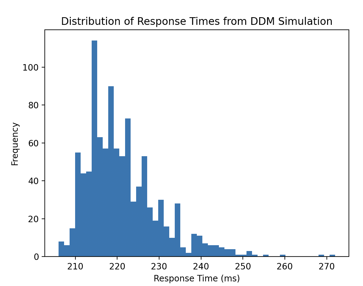
Here’s the distribution of response times generated by our simulation:

DDM simulation time response

And the text output from the simulation:

Mean Response Time: 221.39 ms
Proportion of 'Upper Boundary' Choices: 1.00

Explaining the Results

The histogram above shows the distribution of response times from our DDM simulation. As you can see, it’s positively skewed, meaning there are more fast responses and fewer very slow responses. This is a characteristic pattern often observed in empirical decision-making data and is well-captured by the DDM.

The output Mean Response Time: 221.39 ms tells us that, on average, it took approximately 221 milliseconds for a decision to be made in our simulated trials.

The Proportion of 'Upper Boundary' Choices: 1.00 is particularly interesting. It indicates that in all 1000 simulated trials, the evidence always reached the upper boundary. This is a direct consequence of our chosen parameters:

Effective Drift (v_sensitivity * signal_strength = 0.5): A positive effective drift means there’s a consistent push towards the upper boundary.
Starting Point (z = 10): We started the evidence accumulation significantly closer to the upper boundary (a = 20) than the lower boundary (-a = -20). This initial bias gives a strong advantage to the upper choice.

Because the drift is positive and the starting point is biased, the evidence always accumulated enough to cross the upper threshold before the lower one. If we were to change these parameters (e.g., set z to 0 for no initial bias, or use a negative signal_strength), we would start to see choices for the lower boundary as well.

For more advanced DDM modeling in Python, I highly recommend checking out the HDDM and PyDDM libraries.

Applications in Computational Psychiatry

So, how is this useful in the real world? The DDM provides a powerful lens through which to understand decision-making deficits in various mental health conditions.

ADHD: Individuals with ADHD often exhibit more impulsive decision-making. In the context of the DDM, this can be modeled as a lower decision threshold (a). They require less evidence to make a choice, which can lead to faster but more error-prone decisions. Some research also suggests a lower sensitivity (v), indicating less efficient evidence accumulation.
Borderline Personality Disorder (BPD): BPD is often characterized by emotional impulsivity. Studies have used the DDM to show that in emotionally charged situations, individuals with BPD may have a lower decision boundary, leading to impulsive choices driven by their emotional state.

By fitting the DDM to behavioral data, researchers can gain insights into the underlying cognitive processes that are affected in these disorders. This can help in developing more targeted and effective treatments.

Conclusion

The Drift-Diffusion Model is a prime example of how we can use computational tools to peek under the hood of the human brain. For software engineers, it’s a familiar concept: a model that takes inputs, has parameters, and produces outputs. By understanding and applying these models, we can contribute to the exciting and impactful field of computational psychiatry, helping to “debug” the most complex system we know: the human mind.

I hope this post has piqued your interest in this fascinating field. Stay tuned for more posts in this series as I continue to explore the code behind the brain!