Predictive Minds: How Our Brains Code the Future (and Why it Matters for AI)

Astronaut and brain

Hey everyone! Following up on my last post about the Hierarchical Gaussian Filter (HGF), let’s dive into another powerful framework that underpins much of modern computational neuroscience: Predictive Coding.

If you’re a software engineer, you’re already familiar with systems that generate, process, and react to data. Well, your brain is the ultimate data engine, but it’s not just passively receiving information. It’s an active, relentless prediction machine, constantly trying to guess what’s coming next and only bothering to process the ‘surprises’.

This isn’t just a fascinating biological quirk; it’s a profound computational principle with huge implications for artificial intelligence, robotics, and even our understanding of mental health.

The Brain as a Prediction Machine: An Engineer’s Perspective

Imagine designing a highly efficient data processing pipeline. Would you want it to process every single byte of incoming data with equal scrutiny? Probably not. You’d want it to focus on what’s new, what’s unexpected, what deviates from the norm.

This is precisely how your brain operates, according to Predictive Coding. Instead of being a passive receiver of sensory input, your brain is an active generator of hypotheses. It builds sophisticated internal “generative models” of the world, constantly using them to predict what it expects to see, hear, and feel.

What gets processed and propagated through the system isn’t the raw sensory data itself, but the prediction errors – the discrepancies between what was predicted and what actually happened. Think of it like an advanced anomaly detection system for your reality model. Only the “failed tests” (prediction errors) need immediate attention.

Core Principles of Predictive Coding

Let’s break down the key components:

1. Generative Models: Our Internal Simulators

Our brains are constantly constructing and refining internal models of the world. These aren’t just static databases; they are generative. This means they can be run “forward” to simulate or predict what sensory input should look like.

Engineer’s Analogy: Imagine a game engine that can render a scene based on a world state. Your brain has something similar, but for every aspect of your perception.

2. Prediction and Prediction Error: The Core Loop

At every moment, your brain’s generative models are making predictions about upcoming sensory data.

Prediction: This is the brain’s best guess about what’s about to happen. These predictions flow down the cortical hierarchy, from abstract concepts (e.g., “I am in my kitchen”) to concrete sensory details (e.g., “I expect to see the specific pattern of light from my window”).
Prediction Error ( $\\delta$ ): When the actual sensory input deviates from the brain’s prediction, an error signal is generated. $\delta = \text{Sensory Input} - \text{Prediction}$ These error signals are the only bits of information that flow up the cortical hierarchy, telling the higher levels, “Hey, your prediction was off!“

3. Minimizing Prediction Error: Learning & Action

The brain’s fundamental goal is to continuously minimize prediction error. It has two main strategies for this:

Updating Internal Beliefs (Learning): The brain can adjust its internal model or its current belief about the world to better explain the discrepancy. This is how we learn. If you initially predict a cat but then hear a bark, the prediction error drives you to update your belief to “dog.”
Acting on the World (Action): Sometimes, it’s easier to change the world to match your predictions. If your brain predicts that your hand will pick up a cup, but your hand isn’t moving, there’s a huge prediction error. To resolve this error, your brain sends motor commands to move your hand, thereby making the sensory input match its prediction.

4. Precision Weighting: Managing Uncertainty

Not all prediction errors are created equal. The brain ‘weights’ prediction errors based on their precision (how reliable or certain they are).

Engineer’s Analogy: Think of a Kalman filter, where you weigh new evidence by how reliable it is. If you’re in a dark, noisy room, your visual input has low precision. A small error might be ignored. In a well-lit room, a clear but unexpected visual input (a high-precision error) will drive a much larger update to your beliefs. This is also how the brain is thought to implement attention.

Code Example: A Simple Predictive Coder in Action

To make these concepts concrete, let’s build a simple agent from scratch using just NumPy. This code is perfect for a blog post because it transparently shows the core logic without relying on complex libraries.

Our scenario: An agent exists in a world where it tries to predict a single value. For the first 100 moments, this value is stable, but then it suddenly changes. We’ll watch how the agent’s internal belief adapts.

import numpy as np
import matplotlib.pyplot as plt

# This class clearly demonstrates the core principles for your blog post
class SimplePredictiveCoder:
    """
    A simplified model to illustrate the core loop of predictive coding.
    The agent tries to predict a single, continuous value from the environment.
    """
    def __init__(self, initial_belief=0.0, learning_rate=0.1):
        self.belief = initial_belief      # The agent's internal model of the world state
        self.learning_rate = learning_rate # How quickly the agent updates its belief

    def predict(self):
        """Generates a prediction based on the current belief."""
        # The prediction is simply the current state of the internal model.
        return self.belief

    def update(self, sensory_input):
        """Processes sensory input, calculates error, and updates the belief."""
        # 1. Generate a prediction from the internal model
        prediction = self.predict()

        # 2. Calculate the Prediction Error: the difference between reality and prediction
        prediction_error = sensory_input - prediction

        # 3. Update the belief to reduce future error
        # The belief is moved in the direction of the error, scaled by the learning rate.
        self.belief += self.learning_rate * prediction_error

        # Return key values for plotting
        return prediction, prediction_error

# --- Simulation ---
# We will simulate an environment that suddenly changes
n_trials = 200
true_value = np.zeros(n_trials)
true_value[:100] = 0.2  # The world has a value of 0.2 for the first 100 trials
true_value[100:] = 0.8 # The world's value suddenly changes to 0.8

# Add some noise to the sensory input to make it realistic
noisy_input = true_value + np.random.normal(0, 0.1, n_trials)

# Initialize our agent
agent = SimplePredictiveCoder(initial_belief=0.5, learning_rate=0.05)

# Store the history of the agent's mental states
belief_history = []
prediction_history = []
error_history = []

# Run the simulation loop
for i in range(n_trials):
    prediction, prediction_error = agent.update(noisy_input[i])
    belief_history.append(agent.belief)
    prediction_history.append(prediction)
    error_history.append(prediction_error)

# --- Visualization ---
fig, ax = plt.subplots(2, 1, figsize=(12, 8), sharex=True)
fig.suptitle("Predictive Coding Principle: A Simple Agent Learns a Volatile World", fontsize=16)

# Plot 1: Beliefs and Reality
ax[0].plot(true_value, 'k--', lw=2, label="True World State")
ax[0].plot(belief_history, 'r-', lw=2, label="Agent's Inferred Belief")
ax[0].scatter(range(n_trials), noisy_input, c='gray', alpha=0.3, marker='.', label="Noisy Sensory Input")
ax[0].set_ylabel("Value")
ax[0].set_title("Agent's Belief vs. True World State")
ax[0].legend()
ax[0].grid(True, linestyle=':')

# Plot 2: Prediction Errors
ax[1].plot(error_history, 'b-', label=r"Prediction Error ($\delta$)")
ax[1].set_xlabel("Trial Number")
ax[1].set_ylabel("Prediction Error")
ax[1].set_title("Prediction Error Over Time")
ax[1].axhline(0, color='black', linestyle=':', lw=1)
ax[1].grid(True, linestyle=':')
ax[1].legend()

plt.tight_layout(rect=[0, 0, 1, 0.96])
plt.show()

Dissecting the Output

When you run this code, it produces two plots that perfectly illustrate the theory.

Plot result

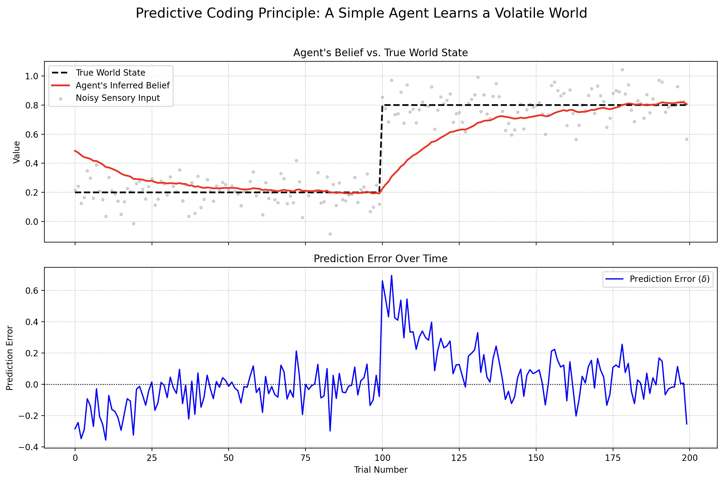
Agent’s Belief vs. True World State (Top Plot): This shows the ground truth (black dashed line) and the agent’s internal belief (red line). Notice how the agent’s belief starts at 0.5 but quickly learns to track the true value of 0.2. When the world suddenly changes at trial 100, the agent’s belief is wrong for a moment, but it rapidly adapts and learns the new reality of 0.8.
Prediction Error Over Time (Bottom Plot): This is the engine of the learning process. The error fluctuates around zero when the agent’s model is accurate. But look at the massive spike at trial 100. This is the “surprise” signal. The sudden environmental change created a huge discrepancy between the agent’s prediction (still around 0.2) and the sensory input (now around 0.8). This large error signal is precisely what drives the rapid change in the agent’s belief, compelling it to update its model of the world.

The Math Behind the Magic

The agent in our code is driven by a few simple but powerful equations that directly mirror the principles we’ve discussed. Let’s denote the agent’s belief at trial $k$ as $b\_k$ .

Prediction: The agent’s prediction, $p\_k$ , is simply its current internal belief. $p_k = b_k$
Prediction Error: The error, $\\delta\_k$ , is the difference between the actual sensory input, $u\_k$ , and the agent’s prediction. This is the “surprise.” $\delta_k = u_k - p_k$
Belief Update: The agent’s belief for the next trial, $b\_{k+1}$ , is calculated by taking the current belief and adjusting it by the prediction error, scaled by a learning rate, $\\alpha$ . $b_{k+1} = b_k + \alpha \cdot \delta_k$

This simple update rule is remarkably powerful. For engineers, it should look very familiar. It’s conceptually identical to gradient descent, where you iteratively update a model’s parameters (our belief) in the direction that minimizes a loss function (our prediction_error). The brain, in essence, is running a continuous optimization algorithm on its model of reality.

Applications and Future Directions

The principles of Predictive Coding are inspiring new approaches across engineering:

Robotics & Control Systems: Building autonomous agents that can predict the sensory consequences of their actions and react robustly to unexpected events.
Generative AI: The core idea of generating outputs (predictions) and then refining them based on an error signal shares conceptual parallels with Predictive Coding.
Anomaly Detection: Identifying system states where observed data strongly deviates from predicted behavior, critical for cybersecurity and infrastructure monitoring.
Neuromorphic Computing: Designing novel computer architectures that emulate brain function for energy-efficient and robust AI.

Further Resources

If you’re hooked and want to dive deeper into this fascinating field, here are some excellent resources to get you started:

Books

Surfing Uncertainty: Prediction, Action, and the Embodied Mind by Andy Clark: A highly accessible and engaging introduction to Predictive Coding from a philosophical and cognitive science perspective. It’s the best place to start for a broad, conceptual understanding.
The Predictive Mind by Jakob Hohwy: A more detailed philosophical exploration of the brain as a hypothesis-testing machine.

Key Papers & Reviews

“A Free Energy Principle for the Brain” by Karl Friston: The foundational (and mathematically dense) paper proposing the Free Energy Principle, which provides a formal framework for Predictive Coding.
“Whatever next? Predictive brains, situated agents, and the future of cognitive science” by Andy Clark: An excellent and more digestible review article that summarizes the core ideas and their implications.

Online Lectures & Videos

Karl Friston: The Free Energy Principle: A lecture from the man himself. It can be challenging, but it provides a direct look into the theory.
Andy Clark: How The Brain Shapes Reality: A talk from Andy Clark that beautifully explains the core concepts of his book in an easy-to-follow format.

Python Libraries & Code

pymdp: A Python library for Active Inference: For those who want to build working models, pymdp is a well-maintained library for simulating active inference agents. Active Inference is the process of minimizing prediction error (or free energy) through both perception and action, making it a direct extension of the principles discussed.

Conclusion: Engineering the Mind

Predictive Coding offers an elegant and powerful framework for understanding the brain. By seeing the brain not as a passive data receiver but as an active prediction engine, we unlock profound insights into how we perceive, learn, and act.

For software engineers, this isn’t just biology; it’s a blueprint for highly adaptive and efficient intelligent systems. The parallels between minimizing prediction error and optimizing a loss function are striking. As we continue to build more sophisticated AI, the brain’s core computational principles will undoubtedly be a key source of inspiration.

Building with AI agents? Helpmaton gives you workspaces, agent memory, budget controls, and webhooks—without the lock-in. It’s source-available so you can self-host when you need to. Quick integrations for Gmail, Notion, Slack, Discord, and others.

Try Helpmaton