Computational Psychiatry: Reinforcement Learning and the Code Behind the Brain's Decisions

In our last post, we took a bird’s-eye view of Computational Psychiatry, touching upon the different modeling techniques used to understand the complexities of the human mind. Today, we’re diving deep into one of the most powerful and influential frameworks in this field: Reinforcement Learning (RL).

As software engineers, we’re used to thinking in terms of algorithms, inputs, and outputs. Reinforcement Learning provides a compelling bridge between this computational mindset and the seemingly chaotic world of human behavior. It allows us to model how we learn, make decisions, and sometimes, how these processes go awry.

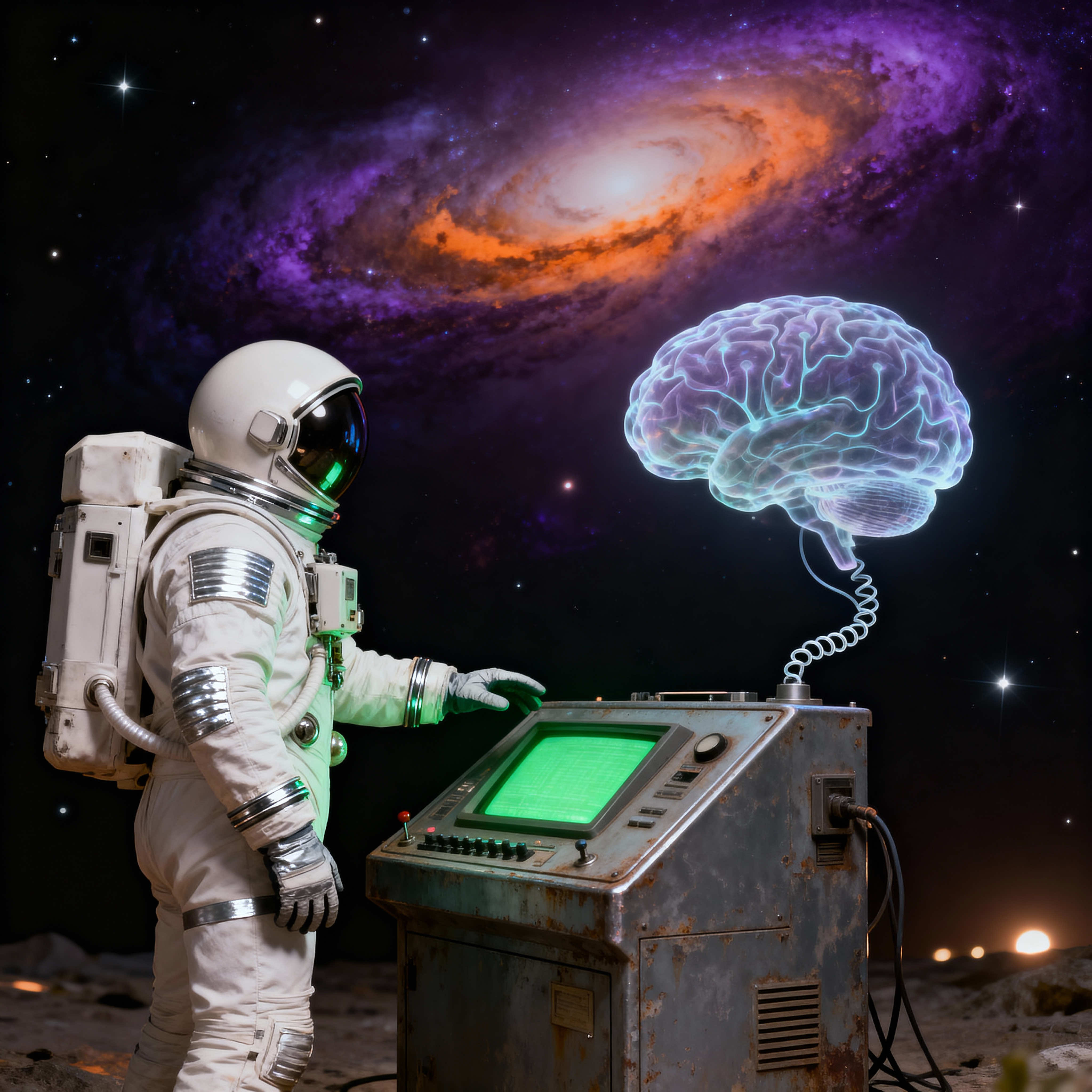
Astronaut analysing the human brain

The Core of Reinforcement Learning: Learning from Consequences

At its heart, RL is about learning from interaction. Imagine an agent (which could be a person, an animal, or a piece of software) existing in an environment. The agent can perform certain actions, and after each action, it receives a reward (or a punishment) and finds itself in a new state. The goal of the agent is to learn a policy—a strategy for choosing actions—that maximizes its cumulative reward over time.

This simple framework can be used to model a vast range of behaviors, from a mouse learning to navigate a maze to a person deciding whether to have a drink or not.

The Math Behind the Magic: Q-learning and Temporal-Difference Learning

For software engineers who love the elegance of mathematics, the beauty of RL lies in its algorithms. Let’s explore two of the most fundamental concepts:

1. Q-learning:

Q-learning is a model-free RL algorithm that aims to find the best action to take in a given state. It does this by learning a “quality” function, known as the Q-function, which estimates the value of taking a certain action in a certain state. The “Q” in Q-learning stands for quality.

The Q-function, denoted as $Q(s, a)$ , represents the expected future reward for taking action a in state s and then following an optimal policy thereafter. The algorithm iteratively updates the Q-values using the Bellman equation:

$Q(s, a) \leftarrow Q(s, a) + \alpha \cdot (r + \gamma \cdot \max_{a'} Q(s', a') - Q(s, a))$

Let’s break down this equation:

$Q(s, a)$ : The current Q-value for state s and action a.
$\alpha$ (alpha): The learning rate, which determines how much new information overrides old information. A high learning rate means the agent learns quickly but may be unstable.
$r$ : The immediate reward received for taking action a in state s.
$\gamma$ (gamma): The discount factor, which determines the importance of future rewards. A value close to 1 means the agent is farsighted and values future rewards highly.
$\max_{a'} Q(s', a')$ : The maximum Q-value for the next state s', representing the best possible future reward.
The term $(r + \gamma \cdot \max_{a'} Q(s', a') - Q(s, a))$ is known as the Temporal Difference (TD) error. It represents the difference between the expected reward and the actual reward.

2. Temporal-Difference (TD) Learning:

TD learning is a more general concept that underlies Q-learning. The key idea of TD learning is to update predictions based on the difference between the predicted value and the actual outcome. This is a form of “bootstrapping,” as it uses the current estimate of the value function to update itself.

The TD error is a crucial concept because it’s believed to be analogous to how our brains learn. The firing of dopamine neurons in the brain has been shown to correlate with the TD error, suggesting that our brains are constantly making predictions and updating them based on the outcomes of our actions.

To make these concepts more concrete, let’s look at a Python implementation of a Q-learning agent navigating a grid world. The agent’s goal is to find the path from a starting point (‘S’) to a goal (‘G’) while avoiding obstacles (’#’).

Instead of just printing the final Q-table (a matrix of numbers), we will do two things to see the result of the training:

Visualize the Policy: We’ll convert the Q-table into a simple visual grid that shows the best action to take from every possible state.
Test the Agent: We’ll run one final episode where the agent uses its learned knowledge to navigate the grid, printing out the optimal path it discovers.

import numpy as np

# Define the environment
# 0: empty, 1: goal, -1: obstacle
grid = np.array([
    [0, 0, 0, 1],
    [0, -1, 0, -1],
    [0, 0, 0, 0]
])

# Define the Q-table
q_table = np.zeros((grid.shape[0], grid.shape[1], 4)) # 4 actions

# --- Hyperparameters ---
learning_rate = 0.1
discount_factor = 0.95
num_episodes = 2000
max_steps_per_episode = 100
epsilon = 1.0               # Exploration rate
max_epsilon = 1.0           # Max exploration rate
min_epsilon = 0.01          # Min exploration rate
decay_rate = 0.005          # Exponential decay rate for exploration prob

# --- Action mapping ---
# 0: up, 1: down, 2: left, 3: right
actions = [(-1, 0), (1, 0), (0, -1), (0, 1)]
action_symbols = ['↑', '↓', '←', '→']

# --- Q-learning algorithm ---
for episode in range(num_episodes):
    state = (0, 0) # starting state
    done = False

    for step in range(max_steps_per_episode):
        # Epsilon-greedy action selection
        if np.random.uniform(0, 1) < epsilon:
            action_index = np.random.randint(4) # Explore
        else:
            action_index = np.argmax(q_table[state]) # Exploit

        action = actions[action_index]

        # Take action, get new state and reward
        new_state = (state[0] + action[0], state[1] + action[1])

        # Boundary check
        if not (0 <= new_state[0] < grid.shape[0] and 0 <= new_state[1] < grid.shape[1]):
            new_state = state # Stay in place if action is invalid

        reward = grid[new_state]

        # Check if goal or obstacle is reached
        if reward == 1 or reward == -1:
            done = True

        # Update Q-table using the Bellman equation
        q_table[state][action_index] = q_table[state][action_index] + learning_rate * \
            (reward + discount_factor * np.max(q_table[new_state]) - q_table[state][action_index])

        state = new_state
        if done:
            break

    # Decay epsilon (exploration rate)
    epsilon = min_epsilon + (max_epsilon - min_epsilon) * np.exp(-decay_rate * episode)

# --- Applying the result ---

# 1. Visualize the learned policy
print("Learned Policy:")
policy_grid = np.chararray(grid.shape, unicode=True)
for row in range(grid.shape[0]):
    for col in range(grid.shape[1]):
        if grid[row, col] == 1:
            policy_grid[row, col] = 'G' # Goal
        elif grid[row, col] == -1:
            policy_grid[row, col] = '#' # Obstacle
        else:
            best_action_index = np.argmax(q_table[(row, col)])
            policy_grid[row, col] = action_symbols[best_action_index]

print(policy_grid)
print("\n" + "="*20 + "\n")

# 2. Simulate the optimal path
print("Optimal Path Simulation:")
path = []
state = (0, 0) # Start state
path.append(state)

for _ in range(max_steps_per_episode):
    # Always choose the best action (no exploration)
    best_action_index = np.argmax(q_table[state])
    action = actions[best_action_index]

    new_state = (state[0] + action[0], state[1] + action[1])
    path.append(new_state)
    state = new_state

    if grid[state] == 1: # Reached goal
        break

# Print the discovered path
path_str = " -> ".join([str(s) for s in path])
print(f"Path: {path_str}")

Interpreting the Results

Running the code above will produce an output similar to this:

Learned Policy:
[['→' '→' '→' 'G']
 ['→' '#' '↑' '#']
 ['→' '→' '↑' '←']]

====================

Optimal Path Simulation:
Path: (0, 0) -> (0, 1) -> (0, 2) -> (0, 3)

The Learned Policy grid clearly shows the agent’s strategy. From the starting position (0,0), it has learned to move right (→). From the cell (1,2), it has learned that the best move is to go up (↑) towards the goal, correctly avoiding the obstacle at (1,3).
The Optimal Path Simulation demonstrates the application of this policy. By starting at (0,0) and always following the best action indicated by the arrows, the agent efficiently finds the shortest, safest route to the goal.

This is the power of Reinforcement Learning: it’s not just about crunching numbers in a table, but about developing a robust strategy to solve a problem based on environmental feedback. This same principle, of learning a policy to maximize rewards, is what allows us to model complex human decision-making.

Applications in Psychiatry: Decoding the Dysregulated Brain

Now, let’s connect these computational concepts to the real world of psychiatry. RL models have been instrumental in helping us understand the mechanisms behind various mental health disorders.

Substance Use Disorder: A Hijacked Reward System

Substance use disorder is a prime example of how the brain’s reward system can be “hijacked.” RL models can help us understand this process in a more formal way.

Altered Reward Prediction Error: In individuals with substance use disorder, drugs can create an abnormally large and positive reward prediction error. This leads to an overvaluation of drug-related cues and actions.
Shift from Model-Based to Model-Free Control: Research suggests that addiction may involve a shift from goal-directed, “model-based” control to habitual, “model-free” control. This means that drug-seeking behavior becomes less sensitive to its long-term consequences and more driven by immediate rewards.

By fitting RL models to the behavior of individuals with substance use disorder, researchers can estimate parameters like the learning rate and discount factor, providing insights into the cognitive deficits that contribute to the disorder.

Depression: The Blunted Reward Signal

Depression is often characterized by anhedonia, the inability to experience pleasure. RL models can help us understand how this symptom might arise from a blunted reward signal.

Reduced Reward Sensitivity: Individuals with depression may have a reduced sensitivity to rewards, leading to a diminished reward prediction error. This can make it difficult to learn from positive experiences and to feel motivated to engage in rewarding activities.
Negative Bias: Depression may also be associated with a negative bias in learning, where individuals are more sensitive to punishments than to rewards. This can lead to a cycle of avoidance and withdrawal.

Further Resources for the Curious Engineer

If this dive into Reinforcement Learning has piqued your interest, here are some resources to deepen your understanding:

Books:
- Reinforcement Learning: An Introduction by Richard S. Sutton and Andrew G. Barto: The definitive textbook on the subject.
Online Courses:
- Coursera’s Reinforcement Learning Specialization: A comprehensive online course from the University of Alberta.
Review Papers:
- Computational Psychiatry: towards a mathematically informed understanding of mental illness: A great overview of the field.
- Reinforcement learning, reward (and punishment), and dopamine in psychiatric disorders: A review focusing on the role of RL in psychiatric disorders.

Conclusion

Reinforcement Learning provides a powerful and intuitive framework for understanding how we learn and make decisions. By applying these models to the study of mental health, we can gain new insights into the computational basis of psychiatric disorders. This is just the beginning of our journey into Computational Psychiatry, and I look forward to exploring more of this fascinating field with you in our next post.